![]()
Disolv
Disolv stands for Dataflow-centric Integrated Simulator Of Large-scale VANETs. Disolv is a VANET simulator implemented in Rust to enable large scale simulation studies of connected traffic applications. This documentation contains the description and the design of the simulator.
Simulator is available as open-source on [GitHub](https://github.com/nagacharan-tangirala/disolv)
Research
Disolv is developed as a tool necessary for my dissertation research. Disolv is used in generating the results in the following publications:
@inproceedings{tangirala2024simulation,
    author = {Tangirala, Nagacharan Teja and Sommer, Christoph and Knoll, Alois},
    title = {{Simulating Data Flows of Very Large Scale Intelligent Transportation Systems}},
    booktitle = {2024 ACM SIGSIM International Conference on Principles of Advanced Discrete Simulation (SIGSIM-PADS 2024)},
    address = {Atlanta, GA},
    month = Jun,
    publisher = {ACM},
    year = {2024},
}

@inproceedings{tangirala2025optimizing,
    author = {Tangirala, Nagacharan Teja and Rishert, Rouven and Sommer, Christoph and Knoll, Alois},
    title = {{Optimizing Very Large Scale ITS Applications With Fast Fitness Evaluation}},
    booktitle = {IEEE Wireless Communications and Networking Conference 2025}
    address = {Milan, Italy}
    month = March,
    publisher = {IEEE},
    year = {2025},
}
Article links and other details about my work are available in my website.
You can learn more about me at [my website.](https://nagacharan.phd)
Capabilities
Disolv is primarily a VANET simulator. It has a simplified implementation of the network protocol so that the user can focus on applications. To demonstrate these strengths, I have developed scenarios that can be found at disolv-scenarios. The documentation will help to understand how to install, compile and use Disolv for different scenarios.
Installation
Disolv is tested in Ubuntu and Macbook Pro. It should technically work with Windows but that is not tested.
Prerequisites
If you are on a new installation of Ubuntu, install the necessary build tools using the command:
sudo apt-get install build-essential
For Mac, you need homebrew and Xcode. Get the XCode from the App store. Install Homebrew with the command:
/bin/bash -c "$(curl -fsSL https://raw.githubusercontent.com/Homebrew/install/HEAD/install.sh)"
Check the latest command from the official Homebrew site if the above command fails.
The rest of the steps are common for any system.
Rust toolchain
Rust toolchain is essential for the simulator to work. At the time of writing this, you can use the following command to install the necessary toolchain:
curl --proto '=https' --tlsv1.2 -sSf https://sh.rustup.rs | sh
Check the official link if the above command fails.
Disolv
- Download the latest main branch using the command:
git clone https://github.com/nagacharan-tangirala/disolv.git
- Navigate to the folder and build all possible executables of the simulator using the command:
cargo build --release
- To build a specific package/executable, use the command:
cargo build --package <package_name> --release
Executables
Disolv is a single repo with multiple executables. Depending on the application, you can select the packages for compilation. More about the executables is described in the Executables section.
Basics
In this section, some preliminary basic ideas are discussed -
Simulation
In general terms, simulation is a representation of a real-world phenomenon. Any process that is observed in the world can be represented in a simulation provided its behavior can be captured in the form of a mathematical model. The evolution of the model over time is observed using simulations.
Time
Models that are defined with changes occuring in continuous time are simulated in the continuous time paradigm. Typically, the models are represented using differential equations. Inherently, the simulation of continuous time models can be expensive in terms of computational cost. While time can be theoretically defined as a continuous quantity, the empirical measurements are often measured at a specific time instants. Based on this idea, time can be modeled as a discrete quantity in the simulations. An added benefit is that the simulations are better in terms of scalability.
Two paradigms are possible with discrete time representation -
Discrete-Time Simulation (DTS)
The models that undergo changes at discrete time instants are called discrete-time simulation models. After every pre-defined time interval, the behavior of the models are updated.
Discrete Events Simulation (DES)
The models are updated whenever a certain event happens at any discrete-time instant. While this is similar to discrete-time simulation, event oriented models can be used to represent inter-dependent behavior of multiple models. An added benefit is that the simulation can skip model updates of time instants with no events.
Agent-based Model (ABM) Simulation
Real-world systems are often a combination of several individual components with their own properties. In ABM simulation, each component and its behavior is modeled as an individual component. Each agent is allowed to behave based on its parameters and can optionally interact with other agents. Although the interaction is optional, typically ABM representation is incorporated where agent interactions are essential modeling requirements. In simple scenarios, the interactions between various components can be easily determined and represented with simple simulation models. However, in most of the real-world processes, the interplay between the components are extremely complex and are hard to determine with simple mathematical equations. In such cases, ABM can be a powerful tool that allows the observation of emergence of the behavior over a period. Time can be represented in either continuous or discrete fashion, although, discrete time is commonly selected for its performance benefits.
Several general purpose ABM simulators exist -
Custom behavior models can be implemented using the frameworks. Some of the processes that can be candidates for simulation are vehicular traffic, mobile network communications, crowd movement simulations, infection propagation simulation etc.
VANET
VANET
VANET stands for Vehicular Ad-hoc Network. In simple words, VANET is a wireless network formed by installing a wireless radio to vehicles. Further, the traffic infrastructure can also be installed with a wireless radio. The interactions between the vehicles and the infrastructure happens through VANET. A wide range of applications are enabled by connecting the vehicles to various components of the infrastructure. Collectively, these applications are called Intelligent Transportation System (ITS) applications. VANET opens up endless possibilities of ITS applications. The introduction of new communication protocols (5G and beyond), vehicles (Autonomous vehicles), and infrastructure (drones) contribute towards explosive growth of possible ITS applications. This necessitates a thorough evaluation of ITS applications. Hence, study of the ITS applications is one of the popular research topics.
VANET Simulations
Due to the futuristic nature of the applications, field trials can be expensive if all possible what-if scenarios must be covered. Simulations are an inexpensive and time-saving approach to perform initial evaluations for ITS applications. Hence, VANET studies are carried out using simulations. The general-purpose simulators are not used because of the sheer complexity involved in the modeling of network and mobility models. For example, in network simulations, the order of agent communication events plays a crucial role in accurately replicating the real-world behavior. Hence, network simulators such as ns-3 employ a combination of ABM with DES, where each entity is represented as an agent and the behavior is triggered at specific time instants through events.
Several open-source simulators are available for VANET studies. Depending on the application, a simple mobility simulator with custom extensions can also be used for VANET studies. Similarly, a network simulator with a simple mobility representation can also be used. Some examples are -
Conceptual Decisions
Disolv is an agent-based model with Discrete-time based progression. A typical VANET simulator can be imagined to be a combination of high-fidelity mobility and network simulators. The problem under study constitutes the application. Together, the architecture looks as shown below:
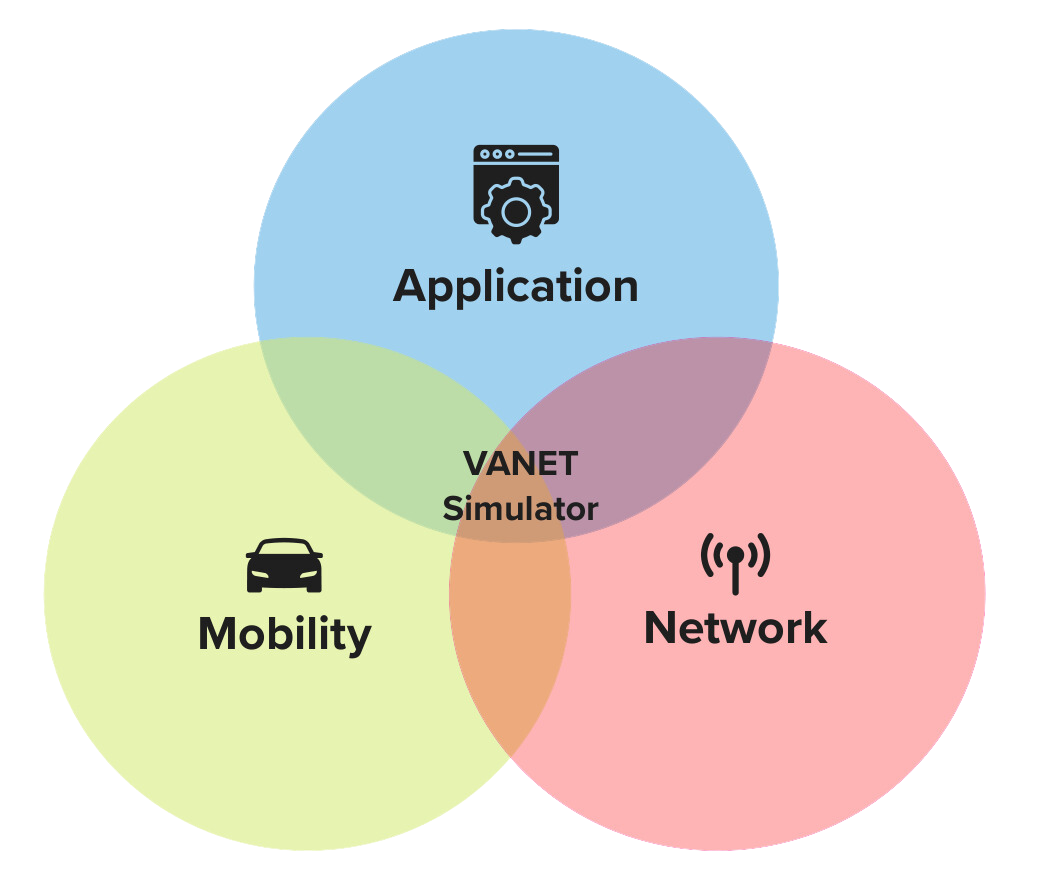
This is how any VANET simulator such as Veins is modeled.
The primary goal of Disolv is to support large-scale evaluation of VANET studies. As a result, all the design decisions of Disolv are oriented towards performance improvements when compared to state-of-the-art VANET simulators. We morph the above simulator idea into an ITS simulator with applications taking the centre stage. There will be mobility and network components, but they are not the main focus of the modeling. Hence, Disolv conceptually looks as shown below:
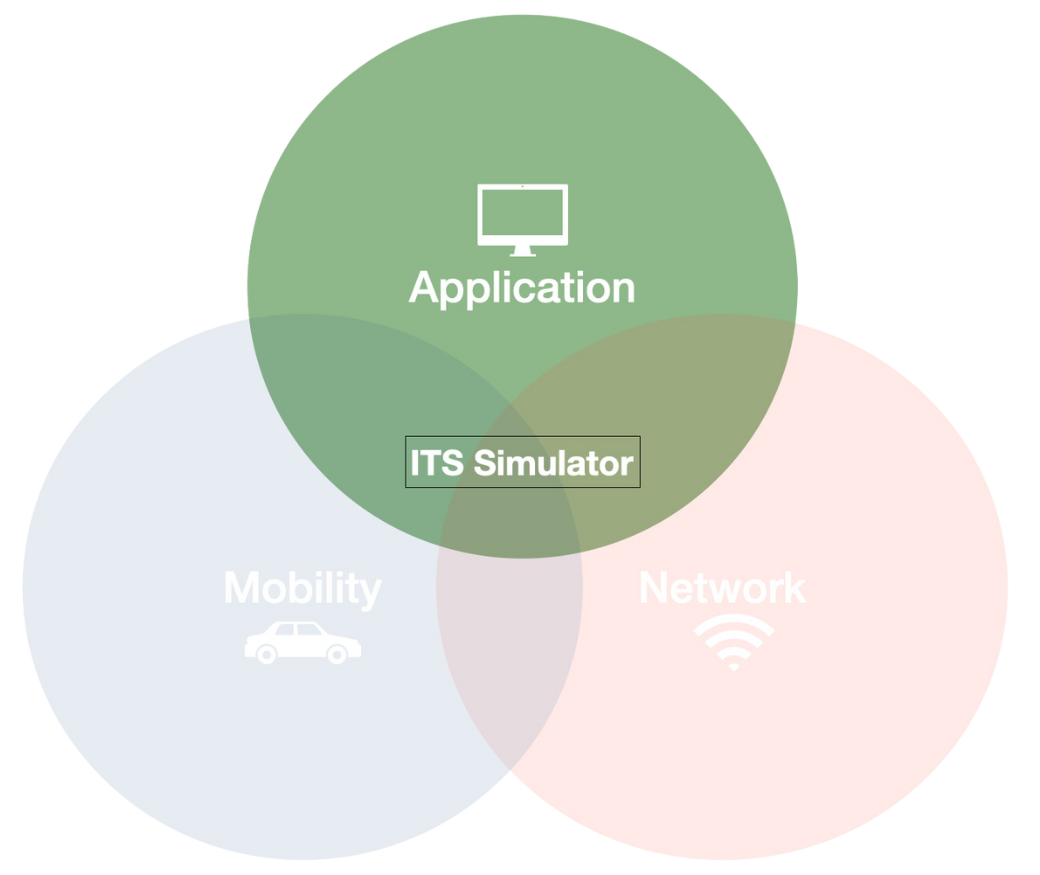
How we reach from the VANET simulator to ITS simulator is the main focus of this section. Several design aspects are incorporated to achieve this and we will look at them in detail.
The details about the choices and their impact on the simulation is compared in the Disolv introductory article published at PADS Conference, 2024.
Mobility
One of the components of a VANET simulator is the mobility component. Mobility modeling is a complex task in itself and has a dedicated community behind it. Some of the mobility simulators are CityMoS, PTV VISSIM, SUMO, MATSim etc. This is unlike the wireless mobile network simulations, where the node mobility can be easily modeled with a random mobility model. Hence, the modeling complexity is high and comes with a performance cost.
On a broad level, ITS applications can be classified into two types. The first type is where explicit control of the vehicles is essential. An example would be truck platooning studies. The second type is where no control of the vehicles is required in the study. For example, network planning studies about the infrastructure placement. Disolv is designed to cater to the applications where explicit control of the vehicles is NOT essential. Hence, the mobility modeling is greatly simplified. Only vehicular traces are sufficient to represent the vehicular mobility. This removes a significant performance overhead from the simulations, thereby allowing the user to spend the computing on their application. If the application is simple enough, then it allows room for extensive scalability.
The approach restricts the usability of Disolv for the applications that control the vehicles. Fortunately, we cover planning studies category which is one of the majorly studied categories by the community. The introduction of 5G and 6G will further explode the possible studies under the category. AI is expected to be a major player in both network management as well as on the application side. The introduction of smart city paradigm and the continued embracing of its ideas put more onus on mobility to interact with other smart city systems. This increases the possibilities even more and leads to several new auxiliary use cases that do not require vehicular control. Based on this intuition, we imagine Disolv to remain usable for plenty of use cases.
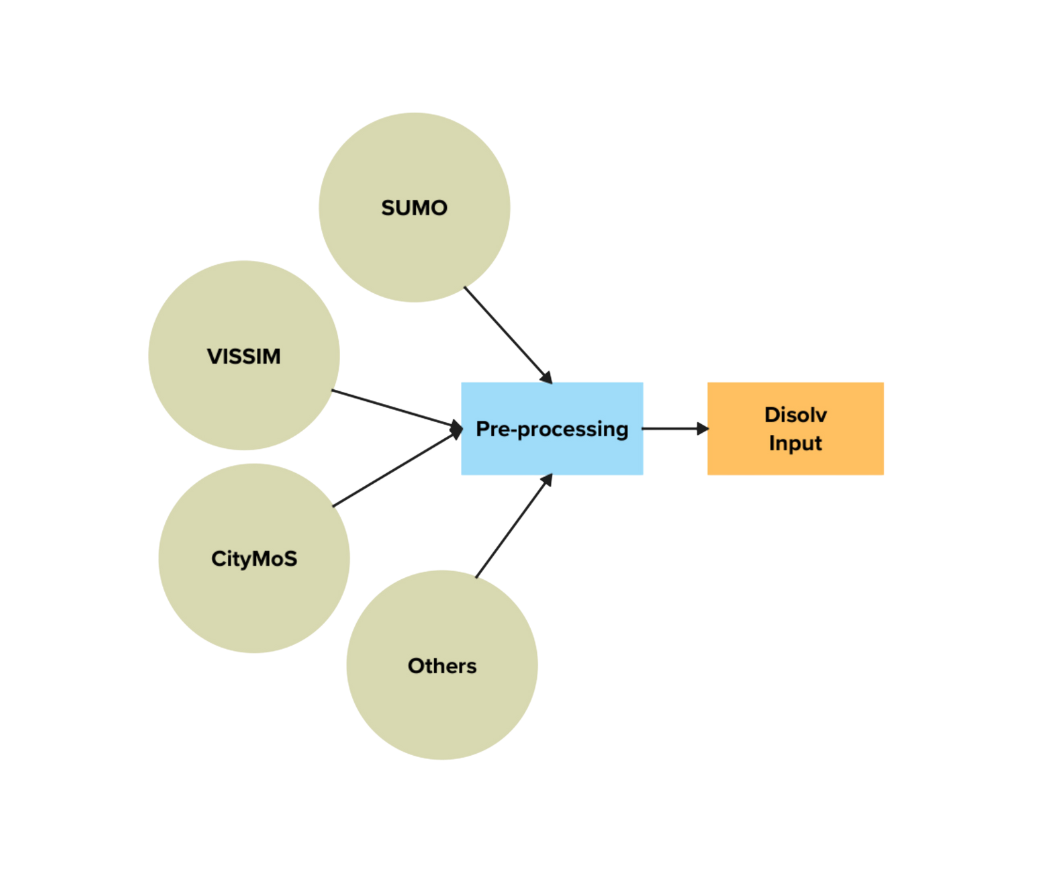
The process of converting a mobility trace to Disolv-readable format is supported by our pre-processing pipeline. Any mobility simulator output can be converted to Disolv-readable format. As of now, SUMO is supported. This has an advantage of feeding a real-world mobility data as an input to the simulator.
Links
The next important component after Mobility is the connectivity. To simulate the communication between agents, each agent must know who is in their vicinity. This is an O(N2) operation because every agent should know about every other agent's position and determine if it is in the vicinity. Because of the motion of the agents, this calculation is essential at each time step. A significant time of the simulation is spent in this operation when the scale of the simulation is extremely large.
Disolv addresses the issue by allowing an input of neighbour information. Similar to vehicular positions, the data for each agent and its neighbours can be fed as an input to the simulation. For the convenience of the users, Disolv comes with an executable that enables preparation of this file. This is a one-time step performed for each simulation and is required whenever there is a change in the positions file.
Links are calculated between two classes of agents. The first class of the agent is the source with respect to which the second class agents are assigned as neighbours. There are several types of links that can be calculated:
Static
If the source and target agent classes are static (RSUs, Edge Servers), then the links need not be calculated for every time step. In such cases, only the links at time step 0 are calculated.
Dynamic
This will calculate links between source and target for all the time step. This is required when one of the agent classes are moving (vehicles, drones).
Unicast
If a source agent can talk to only one agent of the target class at each time step, then such links must be calculated using Unicast method. Depending on the choice, user can assign the nearest target agent.
Circular
This gives all the target agents around a given source agent at each time step. This is similar to a broadcast.
Extensions
Further models can also be easily added for calculating the links.
Real-world Traces
Any real-world traces can also be provided. For instance, an ns-3 scenario can be used to generate the links data. Whenever, there was a packet failure, we can assign no link in this case. What this enables is a realistic communication and vehicular scenario, on top of which other planning applications can be evaluated. In other words, disolv can be used a simulation replay tool.
Streaming
As we saw in the mobility and links sections, disolv needs several input files for a simulation. Because of the large-scale support goals, the size of the individual files can be significantly large. Mobility trace files for a city like Cologne take 20GB. If we add three to five different link files (vehicle-vehicle, vehicle-rsu, rsu-vehicle), then the input size is enormous. On the output side, such large scenarios also generate significant data. This can prove to be detrimental both for the performance as well as the memory.
Disolv is designed to overcome this issue through data streaming abilities. Both the input and output files can be streamed at regular intervals of configurable time steps. Input and output are handled in the form of chunks. This solves the memory issues as the amount of data to be kept in the memory is only one chunk of the entire simulation duration. This is similar to digital twins.
Parquet files are used for their robust and performant behavior. Disolv can be extended to support any file format as requried by the user.
Messages
Any realistic VANET simulator represents the interactions through packets. This is required to also model the failures due to the network resource constraints. Since we are only modeling interactions, packet-level modelling is not necessary. Instead, we model the interactions using a compact structure called Message.
Message is built mainly with the metadata regarding the information that is transmitted. It contains the statistic such as size, counts, type regarding the data. Although this leads to unrealistic network, application studies that are not focussed on these aspects can reasonably benefit from this simplification. Any forwarded data from the downstream is also aggregated and forwarded to the upstream.
For instance, consider the scenario where vehicles are uploading images to the RSU. RSUs are all connected to a central entity that is responsible to collect the images from the vehicles. Disolv can model this scenario. Vehicles can upload their data to the nearest RSU as they travel along the network. RSUs collect all the data that the vehicles uploaded into a single message and forward that to the controller. If we modelled this in the form of packets, we need too many packet instances to represent the interaction. Instead, we represent all of that with one single message.
Message structure
One message is exchanged between a source and target agent. It contains the following information:
Message = {
    message_type: Enum,
    message_units: List,
    gathered_units: List,
    metadata: Struct,
    actions: List,
}
Message Type
Indicates the message type that is being sent.
Message Units
This is an individual unit of a message that needs to be transmitted. Think of it as a unit of application data. Hence, this is a list to support scenarios where multiple applications want to communicate (voice, data, video).
Gathered Units
These are all the application data that were forwarded by the agents in the upstream/downstream.
Metadata
This contains all the necessary statistics of the message, including size, counts, selected link etc. The metadata is updated based on the message units that are supposted to be followed to the target.
Actions
Actions are integral to the interactions between the agents. Each agent can receive either one or more messages from other agents. What to do with each individual message unit is indicated by the action. For instance, we can ask an agent to consume all image type messages but forward all video message types. This is entirely configurable by the user.
Discrete-time
This follows naturally from all the other design choices we have made so far. Since the interactions are simpler, we don't need discrete-event paradigm and its complexity despite its fidelity guarantees. Agents can interact with each other following weakly-ordered priority scheme through discrete-time paradigm. This essentially means that the agent interaction order can be controlled to only a certain extent. We cannot control that vehicle ID A sends a message before vehicle ID B.
That does not mean that we have no control at all. We can modify order at the agent class level. For example, we can specify that vehicles send their messages first before RSUs do or vice versa for a downstream scenario.
Architecture
Disolv is designed as an ensemble of simulators with preparators and library playing a supportive role. There are two main components in the implementation -
Simulators
These are the crates that result in a binary upon compilation. Each simulator is catered to a specific type of scenario. Depending on the application, the user can choose appropriate simulator to compile. Among all the simulators, there is a lot of redundant logic that is crucial for the correct operation of simulator. Such core logic is extracted into its own library crate.
Library
This is the backbone of the simulator containing all the primitive definitions and the trait declarations. The implementation details of the library are further segregated into multiple crates according to the function. Library is designed to be as abstract as possible to support multiple simulation executable files to be built on top of them.
Preparators
These are used to prepare appropriate input files for the simulators. They take input of various kinds and convert them into simulator-readable formats. Earlier, these were implemented in Python. However, due to performance reasons, they are now implemented using Rust.
Library
Library contains the implementation that all the simulators can use. Because of the abstract nature, most of the following crates are used by all the simulators. Only the preparation crates do no use the entire available library crates.
Core
Contains the core logic of the scheduler and the agent definitions according to the ABM.
Models
Contains logic to control the model definitions in the rest of the simulator and provides some implementations of the core models that are common for all simulators.
Input
Contains code to read the input data in the form of parquet files.
Output
Contains code to output data from any of the simulators.
Runner
Contains the code that is responsible to run the given ABM scheduler.
Producers
These are responsible for generating the input files for simulations. Disolv needs three main input data:
Positions
Location data or traces of vehicles and infrastructure is essential to support VANET simulation.
Activation
The time period for which an agent is active in the simulation must be given as input. Positions do this calculation because it goes hand-in-hand with the trace data.
Links
The neighbor information for all agents is required to simulate interactions.
Pipeline
The first entry point is the positions producer. Positions will produce the positions and activation data. Next is the links, which will use the data generated by the positions and creates links data. The combined output will then form the input to Disolv.
Links
This is used to generate link files necessary for Disolv simulation.
Positions
Simulators
V2X
This executable runs the V2X scenarios.
FL
This executable runs the Federated Learning scenarios.